Moody Chart Calculator
Find the Darcy friction factor for any pipe flow condition. Enter your Reynolds number and relative roughness. The calculator solves the Colebrook-White equation and plots your result on an interactive Moody diagram.
Calculate Friction Factor
Results
Moody Chart
Lines show friction factor curves for different relative roughness (ε/D) values.
How to Use the Moody Chart Calculator
You only need two values to get a friction factor: Reynolds number and relative roughness. Here is how to find each one.
Step 1: Calculate Your Reynolds Number
Use Re = ρVD/μ, where ρ is fluid density (kg/m³), V is flow velocity (m/s), D is pipe inner diameter (m), and μ is dynamic viscosity (Pa·s). For water at 20°C, ρ = 998 kg/m³ and μ = 0.001 Pa·s. Not sure of your values? Check our Reynolds number guide for a step-by-step walkthrough.
Step 2: Find Your Relative Roughness
Divide the absolute roughness of your pipe material (ε) by the pipe inner diameter (D). The table in the next section gives you ε values for common materials. For a 100 mm commercial steel pipe, that is 0.046 mm / 100 mm = 0.00046.
Step 3: Read the Result
Enter both values above and click Calculate. The calculator returns your Darcy friction factor and marks your operating point on the Moody diagram. You can then use that friction factor in the Darcy-Weisbach equation to find pressure drop.
Understanding the Moody Chart
What Is the Moody Chart?
Lewis Ferry Moody published this chart in 1944 in a landmark paper in the Transactions of the ASME. It plots Darcy friction factor (f) on the vertical axis against Reynolds number (Re) on the horizontal axis, with curves for different relative roughness values. Engineers use it to solve pipe flow problems without iterating the Colebrook-White equation by hand. You can read the original 1944 Moody paper in the ASME Digital Collection.
The Colebrook-White Equation
The chart is a graphical solution to the Colebrook-White equation, which covers the full turbulent flow regime:
This equation is implicit, meaning f appears on both sides. Our calculator solves it using Newton-Raphson iteration, which converges in 3 to 5 steps. For a simpler explicit approximation, the Swamee-Jain equation gives results within 3% for most engineering conditions.
Flow Regimes Explained
Where your operating point falls on the Moody diagram determines which equation applies.
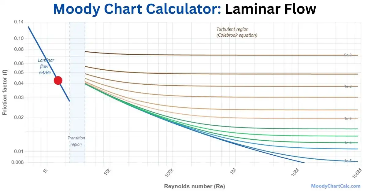
Laminar flow (Re below 2,300) produces smooth, parallel fluid layers. Friction factor follows f = 64/Re, a straight line on the log-log chart. No roughness term is needed because the viscous sublayer covers the pipe wall entirely.
Transitional flow (Re between 2,300 and 4,000) is unstable. Friction factor can vary unpredictably in this zone, so engineers typically design to stay out of it.
Turbulent flow (Re above 4,000) is where most real piping systems operate. Friction factor depends on both Re and relative roughness. At very high Re, the curves flatten and friction factor becomes roughness-dependent only. This is the fully rough turbulent zone.
Pipe Material Roughness Values
Your pipe material sets the lower boundary for friction factor. Use these values to find your relative roughness. For a deeper comparison of materials and their impact on system pressure loss, see our pipe roughness guide.
| Material | Absolute Roughness ε (mm) | Typical ε/D | Common Use |
|---|---|---|---|
| Drawn Tubing / PVC | 0.0015 | 0.000005 | Instrumentation, chemical lines |
| Commercial Steel | 0.046 | 0.00015 | General industrial piping |
| Galvanized Iron | 0.15 | 0.0005 | Water distribution, HVAC |
| Cast Iron | 0.26 | 0.00085 | Municipal water mains |
| Concrete | 0.3 to 3.0 | 0.001 to 0.01 | Stormwater, large culverts |
| Riveted Steel | 0.9 to 9.0 | 0.003 to 0.03 | Older industrial ducts |
Source: Engineering ToolBox roughness data. Actual values vary with pipe age, coating, and installation conditions.
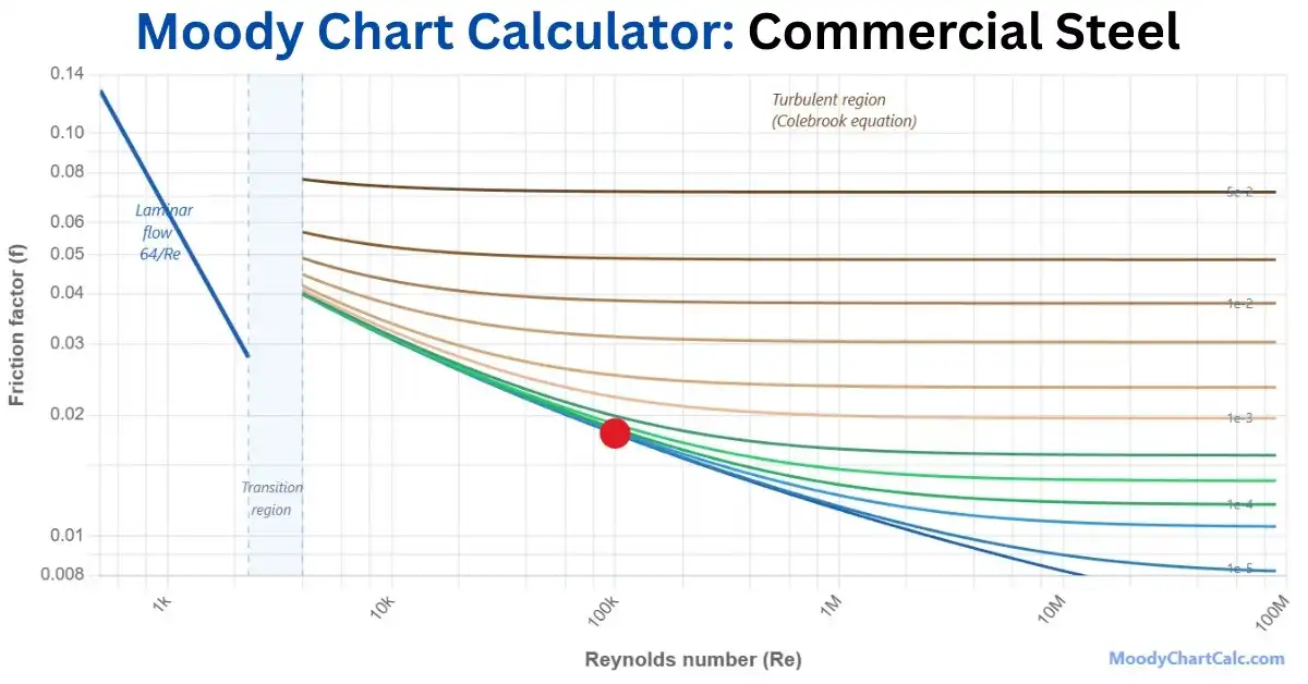
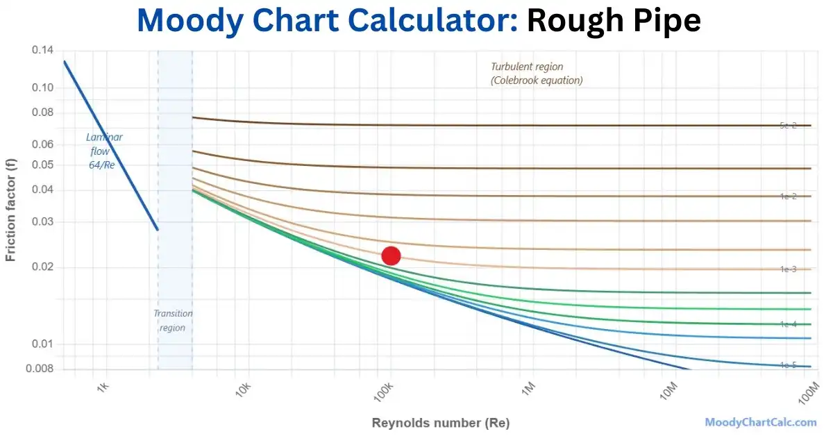
Example Moody Chart Calculations
Below are visual examples of Moody Charts for different pipe conditions. Each example demonstrates how friction factor varies with Reynolds number and relative roughness.

Watch: Moody Chart Explained
Learn how to read the Moody Chart and calculate friction factor.
Using Friction Factor in the Darcy-Weisbach Equation
Once you have your friction factor, you can calculate pressure drop or head loss across any pipe segment. The Darcy-Weisbach equation is the standard method in fluid mechanics:
Where ΔP is pressure drop (Pa), f is the Darcy friction factor, L is pipe length (m), D is inner diameter (m), ρ is fluid density (kg/m³), and V is mean flow velocity (m/s). In head loss form:
The Darcy-Weisbach equation applies to any fluid, any pipe diameter, and any flow velocity. That makes it more versatile than the Hazen-Williams formula, which only works for water. For a side-by-side comparison, read our Darcy-Weisbach vs Hazen-Williams article.
Example Calculation
You have a 50 m long, 100 mm diameter commercial steel pipe carrying water at 2 m/s. Fluid density is 998 kg/m³.
First, calculate Re: Re = 998 × 2 × 0.1 / 0.001 = 199,600. That is turbulent flow.
Relative roughness: 0.046 mm / 100 mm = 0.00046.
Enter those values above. The calculator returns f ≈ 0.0183.
Pressure drop: ΔP = 0.0183 × (50/0.1) × (998 × 4/2) = 18,267 Pa, or about 1.83 m of head loss.
Where Engineers Use the Moody Chart
Friction factor shows up in any problem that involves fluid moving through a pipe. Here are the main application areas.
HVAC and Building Services
HVAC designers use friction factor to size ductwork and chilled water pipework. Getting it wrong means either undersized pipes that cause noise and poor performance, or oversized pipes that waste material and space. The ASHRAE Handbook of Fundamentals uses Darcy-Weisbach as its primary method for duct and pipe sizing.
Water Supply and Municipal Systems
Water utilities use friction factor calculations to model pressure throughout distribution networks. Older cast iron mains have much higher roughness than new HDPE pipes, which directly affects pump sizing and service pressure. Our real-world applications article covers a municipal water case study in detail.
Oil and Gas Pipelines
Long-distance pipelines require precise friction factor values to determine compressor station spacing and operating pressures. Even a small error in friction factor compounds over hundreds of kilometers. Engineers typically run sensitivity analyses across the full roughness uncertainty range.
Chemical Process Engineering
Process engineers size piping for slurries, solvents, and corrosive fluids where viscosity and roughness change over the life of the plant. The Moody Chart applies as long as the flow is single-phase and fully developed.
Pump and System Curve Analysis
The system curve in a pump selection plot comes directly from friction factor calculations at different flow rates. Where the pump curve intersects the system curve is your operating point. Use our calculator to check how friction factor changes as flow increases before you finalize pump selection.
Darcy Friction Factor vs Fanning Friction Factor
This is one of the most common sources of error in pipe flow calculations. The Darcy friction factor (f_D) is four times the Fanning friction factor (f_F):
The Moody Chart uses the Darcy friction factor. The Darcy-Weisbach equation also uses it. But some chemical engineering textbooks and references, particularly older ones, use the Fanning friction factor instead. Before you apply any friction factor value, check which definition the formula you are using requires. Using the wrong one produces a pressure drop error of exactly 4x. Read our full breakdown in the Darcy vs Fanning guide.
Frequently Asked Questions
What is a Moody Chart?
The Moody Chart is a log-log graph that shows you the Darcy friction factor for pipe flow. You find your Reynolds number on the horizontal axis, follow the curve for your relative roughness, and read the friction factor on the vertical axis. Lewis Ferry Moody published it in 1944 and it remains the standard reference in fluid mechanics.
How do you calculate friction factor?
For turbulent flow, solve the Colebrook-White equation iteratively. For laminar flow (Re below 2,300), use f = 64/Re. Our calculator handles both cases automatically. If you want a quick hand calculation for turbulent flow, the Swamee-Jain equation gives results within 3% without iteration.
What is Reynolds number?
Reynolds number (Re) tells you whether your flow is laminar or turbulent. Calculate it with Re = ρVD/μ, where ρ is fluid density, V is velocity, D is pipe diameter, and μ is dynamic viscosity. Below 2,300 is laminar. Above 4,000 is turbulent. Between those values is the unpredictable transition zone.
What is relative roughness?
Relative roughness (ε/D) is absolute pipe roughness divided by pipe inner diameter. It is dimensionless. In turbulent flow, higher relative roughness means higher friction factor. In the fully rough zone at very high Re, friction factor depends only on relative roughness and becomes independent of Reynolds number.
What is the difference between Darcy and Fanning friction factor?
The Darcy friction factor equals four times the Fanning friction factor. The Moody Chart and the Darcy-Weisbach equation both use the Darcy definition. Some chemical engineering texts use Fanning. Always confirm which definition applies before using a friction factor value in a pressure drop formula.
How accurate is this calculator?
It uses the full Colebrook-White equation with Newton-Raphson iteration, converging to within 0.1% of theoretical values. It covers the complete engineering range of Reynolds numbers (laminar through fully turbulent) and relative roughness values up to 0.05.
Go Deeper: Guides and Tutorials
These articles cover the theory and practical steps behind everything this calculator does.
How to Read the Moody Chart
A step-by-step visual guide to finding friction factor directly from the chart.
Reynolds Number Explained
What it is, how to calculate it, and why laminar vs turbulent matters for your design.
Pipe Roughness: A Practical Guide
Roughness values for every common pipe material and how aging affects them.
Colebrook-White vs Swamee-Jain
When to use the exact iterative equation and when the explicit approximation is good enough.
Darcy-Weisbach vs Hazen-Williams
Two methods, two different use cases. Here is which one to use and why.
Moody Chart in Real Engineering
How HVAC, water utilities, and pipeline engineers apply friction factor in real projects.